Give Your AI Searchable Context: RAG on Postgres with pgvector — A Crash Course
15 Concepts · 80% of Real Use · Built by your agent, not by hand
Imagine you could tell your computer: "Take this folder of documents, stand up a database that understands their meaning, and build me a search where asking for 'the city that never sleeps' returns quotes about New York — even the ones that never name it." And it actually does it.
Three words, in case they're new. A database is a warehouse for data: the building where a business stores its goods, except the goods here are information. SQL is the language you speak to that warehouse — every request to store, find, or change data is a sentence in it. Postgres (the database in this course's title) is one of the most widely used in the world. And an ordinary warehouse can only find a box by its exact label; the one you're about to build finds things by what they mean.
That search-by-meaning system is what this course teaches — and here's the twist: you won't write the SQL by hand; Claude Code or OpenCode builds all of it. Your job is to know enough about Postgres and pgvector (the add-on that gives it that power) to give clear instructions and to judge whether the agent got it right. That second part is the whole skill — and by the end, you'll know which knobs matter and which to leave alone.
The bigger claim underneath this course is simple: for most applications, Postgres is the AI database. The separate, specialized vector database you've been told you need is, for most teams, one more system to pay for, sync, and break. Your vectors belong next to the data they describe — and by the end, you won't believe that because this course said so, you'll believe it because you built it.
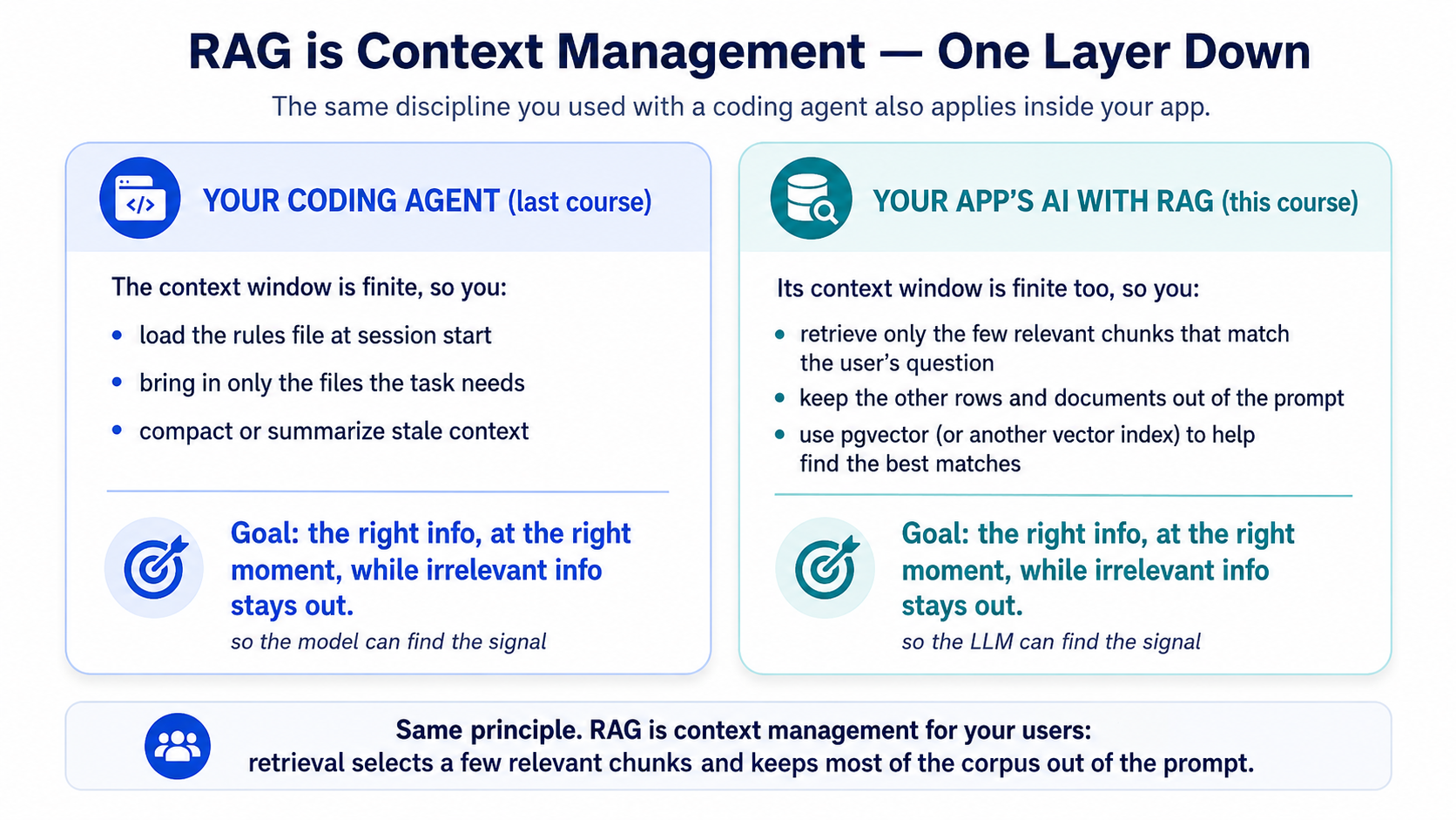
One idea makes this whole course click. An AI model can only pay attention to so much at once: everything it reads to answer you has to fit in its context window, and the more irrelevant material in there, the worse the answer. So the core job in any AI system is getting the right information in front of the model at the right moment, and keeping everything else out. You already do this for your coding agent: a rules file, only the files the task needs. A vector database does the same job for your app's users: out of a million stored rows, it finds the few that match the question's meaning and hands only those to the model. That move has a name — RAG, Retrieval-Augmented Generation — and it is context management, one layer down: what you do for your coding agent by hand, your app does for its users automatically. Every concept here connects back to that.
This course assumes you have done the Agentic Coding Crash Course — you should be comfortable driving Claude Code or OpenCode, using plan mode, and managing context. It also builds on AI Prompting in 2026 — the craft of asking an AI for exactly what you want. If "embedding" and "vector" are brand new to you, don't worry — Concept 2 covers them from zero.
📚 Teaching Aid
View Full Presentation — AI Searchable Context
Two tools, one discipline
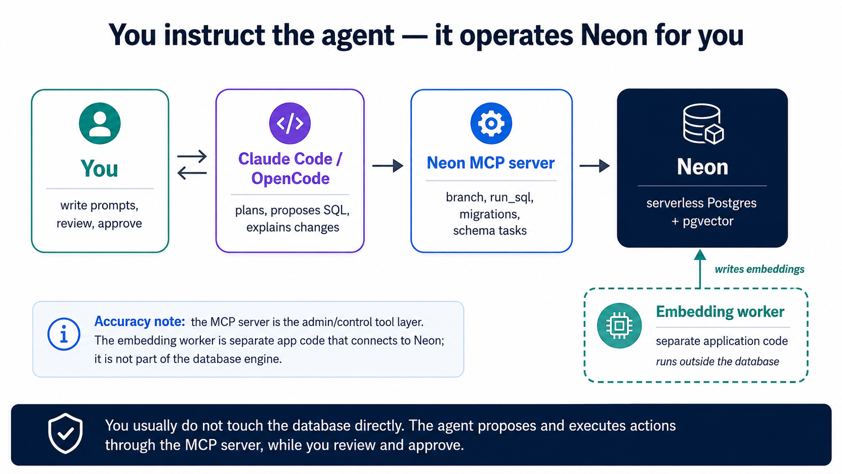
The agent does the driving; your Postgres database is what it drives. The database lives on Neon, a cloud service that runs Postgres for you — nothing to install, no machine to manage (that's all serverless means: it wakes when you use it, sleeps when you don't). The agent operates Neon through the Neon MCP server: it creates the project, opens a branch, runs the SQL, and previews each change on that branch before committing it. You never click around the Neon console or open psql yourself. And the discipline is identical in both tools: Claude Code and OpenCode are equals here — where a command genuinely differs, I call out the difference inline.
What this course covers
| Part | Topic | What you learn |
|---|---|---|
| 1 | Foundations | Your job as the AI engineer, vectors from zero, what Postgres needs to search by meaning, and your agent connected to Neon |
| 2 | Your First RAG | Load your data, split it into pieces, turn each piece into a meaning-vector, search by meaning, and have an LLM answer from it |
| 3 | Making Search Fast | When a slowing search needs an index, how to choose one, and the one speed-vs-accuracy knob that matters |
| 4 | Making Search Good | Measure whether answers are actually right, add filters, mix meaning with exact keywords, wall off each customer's data, and ask your database questions in plain English |
| 5 | Full Worked Example | One complete task — empty database to working RAG — driven in both tools |
| 6 | Ship It as a Tool | Wrap your RAG in an MCP server so any agent — Claude Code, OpenCode, or a Digital FTE you'll build later — can call it |
| 7 | Where It Runs | Test changes on instant copies of your database, keep vectors fresh as data changes, and what's different in production |
| 8 | Hand It to an Agent | Plug your RAG into an agent (OpenAI Agents SDK) — the bridge to the Build AI Agents course |
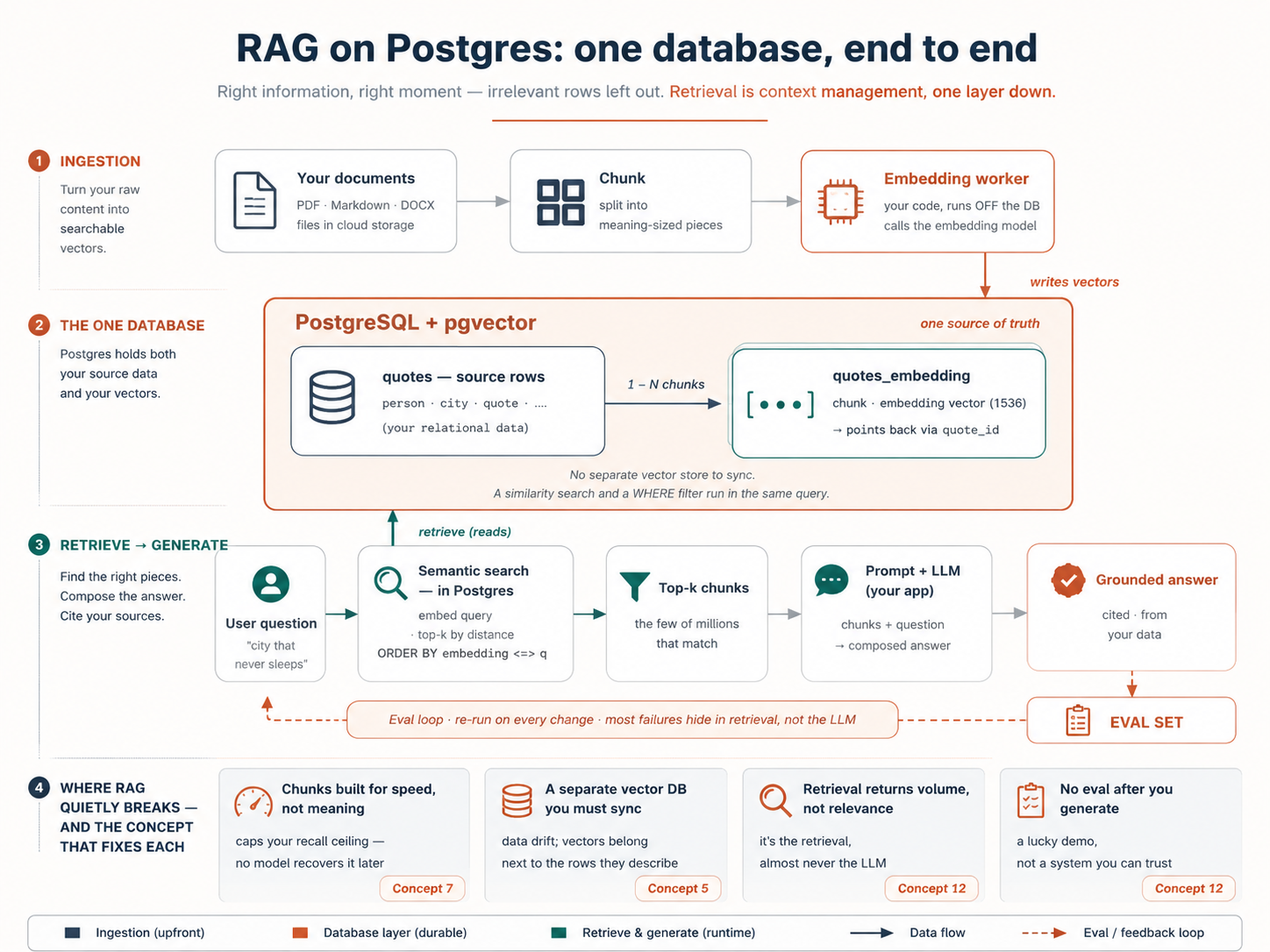
Here's the whole system on one page — the map you'll grow into as each concept lands:
 |
|
By the end you'll have a working RAG project: your docs/ folder of documents loaded into a Neon database with pgvector switched on, a small worker that keeps the meaning-vectors up to date as documents change, a search that finds by meaning, an answer_question() function that answers from your own data, and a report showing whether five test questions come back right. And you won't stop at the easy 80%: you'll have benchmarked an HNSW index from slow to instant, filtered search by category, fused keyword and meaning with hybrid search, and walled one tenant off from another with Row-Level Security — each run for real, measured against your eval set. Optionally, an MCP server hands the whole thing to any agent.
How to read this. Parts 1–2 (Concepts 1–9) plus the worked example in Part 5 are the complete system, end to end — about a 2-hour read at genuine comprehension (more if "vector" is new), plus a few hours at the keyboard for the build. Parts 3–4 (Concepts 10–15) are the tuning layer — what makes search fast (Part 3) and good (Part 4). Read them for the why, then run every one of them: Part 5 ends with a hands-on loop (Steps 5–8) where you build an index benchmark, a filter, hybrid search, and tenant isolation for real, on the data you just loaded. The depth isn't optional reading you might come back to — it's the second half of the build, and everyone does it. Rather build first and read the why after? Jump straight to Part 5.
Set up your environment (once)
Everything you build in this course happens inside one small folder: the course base. It comes pre-wired — your agent already knows how to reach Neon (the cloud database this course uses) and Context7 (live docs lookup, so the agent checks current documentation instead of guessing) — and it ships a short rules file, AGENTS.md, with the project's standing instructions. Your agent reads that file automatically every time it starts, which is why your prompts in this course can stay short.
Download it once; the same folder serves the whole course, the worked example in Part 5 and the MCP server in Part 6 alike. Set it up now or later — the reading itself needs nothing installed.
Unzip it, then open your agent inside the folder:
cd postgres-ai
claude
cd postgres-ai
opencode
One requirement: a capable model. If the agent's first plan ever looks vague instead of specific, switch to a stronger one (Claude Sonnet or Opus, GPT-5, or similar) before going further.
Prep the base (~3 min). The agent does its own setup — you paste one prompt and answer what it asks. Paste this:
Get this base ready: install the skills it lists, set up my
.env, and tell me exactly what you need from me to bring the Neon and Context7 MCP servers online.
Watch for: the agent installs two skills (neon-postgres and mcp-builder), creates .env, then asks you for two things: one API key (the same key covers both embeddings and answers), and one browser click to authorize Neon. The key is free. This course runs on Google Gemini's free tier (no credit card), so the agent points you to aistudio.google.com/apikey; sign in with Google, create a key in about a minute, paste it back, and the agent proves it works on the spot. (Already have an OpenAI key and prefer it? Just say so, and the agent uses that instead; nothing else in the course changes.) Neon is free too; no account yet? Create one right at the authorization screen. If no browser window opens on its own, type /mcp in the agent, pick Neon, and it will start the sign-in for you.
Done when: the skills are installed, .env holds your key and the agent has confirmed it with a quick test call, Neon is authorized, and you've restarted the agent (exit, relaunch) so the new skills and MCP servers load (neither loads mid-session).
Part 1: Foundations
1. What you're actually building (and your job in it)
The most common misconception: building AI applications requires a machine-learning team. It does not. The models are off-the-shelf. The infrastructure is a database you may already run. What's left is the work of an AI engineer — someone who uses AI to build products, rather than a researcher who trains models. That's the role this whole book is preparing you for, and it's very much within reach.
The second misconception is the one this course exists to fix: that you must hand-write all the SQL. You don't. You direct an agent that already knows pgvector's operators and the embedding workflow cold. Your value moves up the stack — from typing CREATE INDEX to deciding which index, from writing the query to judging whether the results are any good.
That changes what "knowing this material" means. You're not memorizing syntax; you're building enough of a mental model to:
- give the agent a precise instruction ("store the embedding in the same table, use cosine distance, index it with HNSW"),
- read back what it produced and spot when it's wrong,
- and decide the architecture choices the agent shouldn't make for you.
This is the same plan-then-execute habit from the coding course — and here it matters even more, because the agent is about to make decisions (which extension, which index, which distance function) that are expensive to undo once you have data.
The mindset shift: stop asking "what's the SQL for semantic search?" Start saying "build me semantic search over this table; here are my constraints; show me the plan first."
There's a bigger name for this. In the book's terms, the database you're about to build is a system of record for the agent era — the authoritative ground truth your agents read from, write to, and verify against. Jensen Huang's argument is that agents don't remove the need for a system of record; they depend on one. Without authoritative ground truth an agent hallucinates; with it, it executes. RAG on Postgres is how you hand an agent that ground truth — which is exactly why the rest of this course treats retrieval quality as the thing that decides whether the agent can be trusted.
Take this literally for the rest of the course: every SQL block below is shown so you can read and judge what the agent produced, not so you can type it. Knowing how to read it is what lets you catch a wrong distance function or a missing filter before it ships.
2. Vectors and embeddings, in one minute
If "vector" and "embedding" are new, here is everything you need to start.
A vector is just a list of numbers — [0.021, -0.88, 0.14, …]. An embedding model takes a piece of content (a sentence, a paragraph, an image) and turns it into one of these lists. The trick is that the list captures the meaning of the content: two pieces of text that mean similar things get lists of numbers that sit close together. Two phrases that mean the same thing — "the city that never sleeps" and "New York's restless streets" — land near each other even though they share no words.
A vector database is just a system that stores these lists and finds the closest ones to a given list, fast. That's it. When a user asks a question, your app embeds their question into a vector, then asks the database: "which stored vectors are nearest to this one?" The nearest ones are the most semantically relevant — and that is how your app fetches the right context to hand an LLM. (See the opening diagram: this is context management for your users.)
You do not need to understand how the embedding model works internally any more than you need to understand how a JPEG compresses an image. You need to know it exists, that it converts content to meaning-vectors, and that closeness equals similarity.
Open a session and ask your agent: "In plain language, explain what an embedding is, then show me two short sentences that would have nearby vectors and two that would be far apart — and why. Then the fun one: would a famous song or nickname for my city land near the city's name, even if the words never say it?" Reading its answer is a faster gut-check on your own understanding than re-reading this section.
3. The extensions — and what you get on Neon
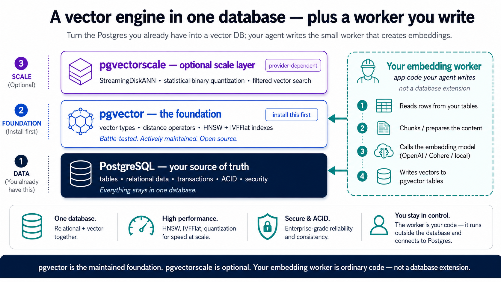
Postgres becomes a vector database through extensions — add-ons that give it new powers without giving up what Postgres already does well (transactions, joins, reliability, SQL). For this whole course there is really only one to learn: pgvector. It adds three things — a vector type to store embeddings, distance operators to compare them, and indexes to search them fast — and on Neon it ships pre-installed, so one statement switches it on. That is your complete RAG engine. Hold just that. (Two footnotes you can park: a second extension, pgvectorscale, exists for very large scale — it's the tier you graduate to, not where you start. And the embeddings themselves aren't an extension at all; they come from a small worker your agent writes, built in Concept 6.)
| Extension | What it adds | When you need it |
|---|---|---|
| pgvector | The vector data type, distance operators, and the HNSW + IVFFlat indexes | Always — and on Neon it's pre-installed |
| pgvectorscale | The StreamingDiskANN index, vector compression, high-accuracy filtered search at large scale | Native on TigerData; not on Neon, where it's the tier you graduate to |
The index names in this table — HNSW, IVFFlat, StreamingDiskANN — are just labels for now; Part 3 teaches what they do and when to use each.
On Neon, pgvector is your whole stack. It ships built in, and everything this course does after embedding — semantic search, indexing, evals, filters, hybrid search, RLS, the Part 6 MCP server — is pure pgvector. The embeddings come from the worker (Concept 6), not a managed extension. As for pgvectorscale: it isn't in Neon's vetted set, so treat it as the host you'd graduate to only if you outgrow HNSW — and pgvector plus a worker carries you a long way first. Want the scale tier native from day one instead? That's TigerData Cloud, same workflow throughout — the one note at the end of Concept 4 covers it, and you can otherwise read this whole course as Neon-only.
The one-database payoff still holds: your vectors live next to the rows they describe, so a similarity search and a WHERE price < 2000 AND in_stock filter happen in the same query, on the same source of truth. No second database, no sync pipeline, no data drift. (Hold onto that — it's the whole reason filtered search in Concept 13 is so easy.)
pgvector is a mature, widely used Postgres extension — the stable bedrock this whole course rests on. Everything after embedding (semantic search, indexing, evals, filters, hybrid search, RLS, the MCP server) is pure pgvector.
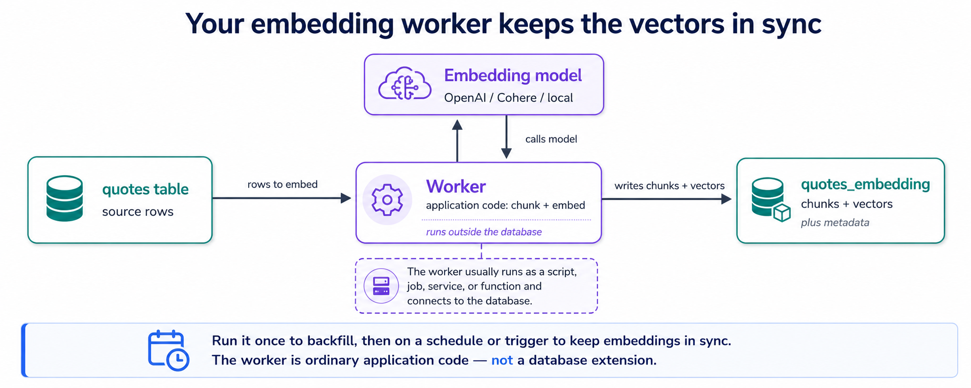
The one thing pgvector doesn't do for you is create the embeddings — calling an embedding model and writing the vectors back. The clean, portable way to do that is a small worker your agent writes: source table → chunk → embed via an API call → write vectors to an embeddings table → search with pgvector. Keeping that work outside the database is the point, not a workaround — a stateful system of record shouldn't depend on a volatile external API, so embedding (and the LLM calls in Concept 9) live in the worker and app layers, where they can fail, retry, and scale without touching your data, and the whole thing ports cleanly to any host or container. (A managed convenience layer once baked embedding into the database — pgai's Vectorizer — but that coupling proved brittle, and its repository was archived by the maintainer in Feb 2026; this course doesn't depend on it.) The worker is a few lines your agent produces and you review. Learn the pattern; it outlives any one package.
4. Connect your agent to Neon
We don't install or run our own database. We use Neon — serverless Postgres with pgvector already built in — and we let the agent operate it through the Neon MCP server. MCP is the same connector mechanism from the coding course; here it hands Claude Code and OpenCode a set of tools (create_project, create_branch, run_sql, get_database_tables, prepare_database_migration, complete_database_migration) so they can manage Neon entirely through natural language. You never open the Neon console or a psql shell yourself. (This course uses Neon as its default host; everything works identically on TigerData Cloud — see "Prefer TigerData?" at the end of this concept.)
One-time wiring. If you started from the course base, the Neon MCP server is already declared in .mcp.json (Claude Code) and opencode.json (OpenCode) — you authorize it once in the browser over OAuth, with no API key to manage. (Wiring it by hand instead is the same single step: add the Neon MCP server to your tool and authorize it.) That is the only manual setup; from here on, everything happens by instructing the agent. Drive it in plan mode:
Using the Neon MCP server, create a project called
agent-factory-ragand enable the pgvector extension on it. Then create a branch calleddevfor us to build on, and save that branch's connection string to.envasDATABASE_URLso the worker and app can read it later (never print my API key). Show me the plan before you run anything.
Then read the plan. What you're checking for:
- It works on a branch, not directly on production. Branching is Neon's superpower: a branch is an instant clone of your whole database (copy-on-write: it stores only what you change, so cloning is free and immediate). The agent makes schema changes on a branch, you preview them, and only then commit to the default branch — the same plan-then-execute discipline, enforced by the platform. (It's also how you'll benchmark indexes and run evals later: branch, test, throw the branch away.)
- It enables pgvector — the one extension this course needs — with a single statement:
CREATE EXTENSION IF NOT EXISTS vector; -- pgvector is pre-installed on Neon; this just switches it on
- For embeddings (Concept 6), the agent builds a small worker — a short Python script or service — that reads new or changed rows, calls the embedding model, and writes the vectors into an embeddings table. It runs off Neon, reaching your branch over its connection string. The embedding provider's API key lives in the worker's environment, never in the database.
You do not need to memorize the MCP tool names or Neon's API. The point of plan mode is that you read the plan, confirm it's working on a branch and enabling pgvector, and then approve. If the plan does something you don't recognize, ask the agent why before saying yes — that question is your real job.
Neon's own guidance is that the MCP server is meant for local development and IDE integrations — it can run powerful operations, so keep it to your dev workflow and review every action the agent proposes before approving. Production changes still go through your normal reviewed migration process.
The course base already includes a short AGENTS.md / CLAUDE.md with the rules this course needs: which Neon branch you're on, that keys live in the environment (never committed), your chosen distance function, and two hard rules — "always make schema changes on a Neon branch and let me preview before committing," and "never run destructive SQL (DROP, TRUNCATE, DELETE without WHERE) without showing me first." Building without the base? Run /init and trim to exactly that.
Everything in this course runs unchanged on TigerData Cloud — the team behind pgvector's companion extensions, who position it as "Agentic Postgres." The agent-driven loop is identical; only the names change:
- Tiger MCP in place of the Neon MCP server. It's built into the Tiger CLI — install it with
tiger mcp install, then drive Tiger Cloud in natural language exactly as above ("create a service, fork it, enable the extensions, show me the plan first"). It even ships Postgres Skills that teach the agent best practices. - Forks in place of branches:
tiger service fork …makes an instant, zero-copy clone — the same fork → test → throw away discipline you'll use for evals and index benchmarks. - pgvectorscale is native (alongside pgvector) — so the StreamingDiskANN "graduate tier" (Concept 11) is in the box from day one, and its index supports vectors up to 16,000 dimensions (big models like
text-embedding-3-largethen need nohalfvec). Your embedding worker runs the same way it does on Neon.
Your embedding worker and the generation step both live in app code — identical to Neon. Rule of thumb: Neon for the simplest serverless start; TigerData when you want pgvectorscale's scale and filtered-search performance without ever migrating.
This course uses Neon for two reasons: a free tier with no credit card, and instant branching the agent drives through the Neon MCP server. Prefer to run Postgres locally (Homebrew, Docker) or on another host? The data side is identical — same CREATE EXTENSION vector, same schema, same worker, same queries; just point DATABASE_URL at your instance. What you give up is the MCP-driven branching (the "branch, test, throw away" move you'll use for indexes and evals), so you'd run those steps directly instead. Everything you learn here transfers unchanged.
Part 2: Your first RAG, built by your agent
We'll build a small, classic example: a table of quotes by historical figures about US cities, then search it by meaning, then have an LLM answer questions over it.
5. The schema: vectors live next to your data
Ask the agent for the source table first. One thing to hold: the meaning-vectors will not live in some separate store — they go in this same database, in the companion table you'll build in the next concept, right beside the data they describe.
Create a
quotestable with columns:person,city, andquote. We'll add embeddings in a companion table next, populated by a small worker — so for now just the source data. Then insert a handful of real quotes about New York, San Francisco, and Chicago so we have something to search.
The table the agent writes will look about like this:
CREATE TABLE quotes (
  id     bigint GENERATED ALWAYS AS IDENTITY PRIMARY KEY,
  person text NOT NULL,
  city   text NOT NULL,
  quote  text NOT NULL
);
The mental model to hold: one source of truth. The quote, who said it, the city, and (soon) its meaning-vector all live in the same database. That's what makes the filtering in Part 4 trivial.
6. Create embeddings — the worker your agent builds
Your quotes table holds text. For the database to search that text by meaning, every piece of it needs a vector — and making those vectors is the one job pgvector doesn't do for you. So the agent writes a small program: the embedding worker. Its whole job is one loop — find quotes that have no vectors yet → split any long text into pieces (chunks) → ask the embedding model for each piece's vector → save the vectors. Run it once and every existing quote is covered; re-run it on a schedule and new or edited quotes get covered too. That is the entire machine.
Where do the vectors get saved? In a second table, the companion table — one row per chunk, each pointing back at the quote it came from. That answers the question everyone asks here (one row, one embedding?): a short quote is one chunk, so one vector row; a long speech becomes several pieces, so several rows. (Why split at all? That's Concept 7, right after this.) Two tables, and they look like this:
quotes  (your source table)        quotes_embedding  (companion table)
┌────┬─────────────────────┐       ┌─────┬──────────┬──────────────┬───────────┐
│ id │ quote               │       │ id  │ quote_id │ chunk        │ embedding │
├────┼─────────────────────┤       ├─────┼──────────┼──────────────┼───────────┤
│ 7  │ a short quote       │ ────→ │ 1   │ 7        │ whole quote  │ [0.02, …] │
│ 8  │ a long speech…      │ ──┬─→ │ 2   │ 8        │ first piece  │ [0.11, …] │
└────┴─────────────────────┘   └─→ │ 3   │ 8        │ second piece │ [0.54, …] │
                                   └─────┴──────────┴──────────────┴───────────┘
  one row per quote                  one row per CHUNK (its own id),
                                     pointing back via quote_id
One decision before the agent builds it: which embedding model turns text into vectors. It's the only choice here that's annoying to reverse, since switching models means re-embedding everything, so it's worth understanding even though the base already picked a sensible default for you. That default is whatever provider you set up: Google's gemini-embedding-001 on the free Gemini path, or OpenAI's text-embedding-3-small if you chose OpenAI. Both run at 1536 dimensions here, both are plenty for most RAG, and Gemini's is free, so you never pick a model name yourself; the base set it to match the key you gave. Two reasons you'd ever stray from the default: your content isn't English (or is deeply specialized, like legal, medical, or code), where a multilingual or domain-tuned model can win; or your evals later show a bigger model genuinely retrieves better. In the worker the model is a single setting, so you test alternatives on your eval set (Concept 12) instead of guessing: shortlist candidates from the MTEB leaderboard (the standard public benchmark for embedding models) and let your data pick the winner.
The dimension fine print (read when you stray from the default)
More dimensions means more storage and memory and slightly slower search. Two practical notes: many modern models let you request fewer dimensions without re-training (this course uses exactly that to pin both providers at 1536), and, a real gotcha, pgvector's HNSW/IVFFlat indexes cap the vector type at 2,000 dimensions (the halfvec type extends that to 4,000), so a full-size 3072-dim model (OpenAI's text-embedding-3-large, or Gemini at full size) would need halfvec or reduced dimensions to be indexable. Staying at 1536 keeps you clear of all this; your agent should flag the cap if you ever raise dimensions, and you should recognize it when it does. (On TigerData, pgvectorscale's StreamingDiskANN index supports vectors up to 16,000 dimensions, so the limit rarely bites.)
First, give the code a home — one Python project, managed by uv (the Python project manager; the agent knows it, and routing every dependency through it keeps the project reproducible):
Set up a Python project in this folder with uv. From here on, add every dependency and run every script through uv.
Then have the agent build the worker and its table:
Create a companion table
quotes_embeddingwith a foreign key toquotes, the chunk text, and anembedding vector(1536)column. Then write a small embedding worker that finds quotes with no current embedding, chunks thequotetext, embeds each chunk with the course's embedding model, and inserts the vectors intoquotes_embedding. Run it once to backfill, show me how to confirm the rows landed, and explain how I'd schedule it. Read the API key from the environment.
Watch for: the agent creates the companion table (the exact shape in the diagram above), runs the worker once, and shows you the vector rows that landed. If the worker dies on its first embedding call with a 401 or 429, nothing in your code is broken; it's the key, and you most likely caught this already at setup, where the agent test-called it. On Gemini, re-copy the free key from aistudio.google.com/apikey; on OpenAI, a brand-new account often needs a payment method before it will embed. A 429 is a rate limit, so wait a moment and re-run. Fix the key, then re-run. If instead you see expected 1536 dimensions, got 3072, the embedding call didn't request 1536 dims — both providers default to a larger vector, so the call must ask for 1536 to match the vector(1536) column; the base worker already does this, so that error means a hand-edited call dropped it. Done when: every quote has at least one row in quotes_embedding, and you know the one command that re-runs the worker.
The simplest version polls: the worker re-runs on a schedule and re-embeds rows whose text changed. Want change-driven updates instead? An INSERT/UPDATE trigger can mark a row dirty — flagging "this one needs a fresh embedding" — and the worker picks those flagged rows up on its next pass. If you ever run more than one copy of the worker to keep up, they mustn't grab the same row twice; Postgres handles that for you, handing each worker a different batch of unclaimed rows (the SKIP LOCKED trick). So the to-do list of rows-needing-embedding is just an ordinary Postgres table — no separate queue service to run, the same one-database payoff as your vectors. Either way the trigger only flags; the embedding call still happens out in the worker, and the database itself never calls the embedding API.
The same worker pattern embeds documents, not just short fields — point it at PDFs, DOCX, or files in cloud storage (an Amazon S3 bucket, for example) and have it parse, chunk, and embed them into the same companion table. And because the model is one setting in the worker, you can swap providers (Gemini, OpenAI, Cohere, Voyage, a local model) to test which retrieves best on your data, the model experiment above.
The worker calls an external embedding provider, so it needs that provider's API key. The key belongs to the worker's environment (or your cloud provider's secret store), never hard-coded in SQL or committed to your repo. Tell your agent explicitly: "read the API key from an environment variable, never write it into a file we commit." Then verify the diff before you approve. Switching embedding providers later (between Gemini and OpenAI, or to Cohere, Voyage, a local model) is a one-line change in the worker; the rest of your app doesn't move.
7. Chunking — the lever that sets your ceiling
Chunking is one step inside your worker — and, quietly, the most important one. A long document embedded as a single vector turns into mush — one blurry average of everything it says — so you split it into smaller chunks, and each chunk gets its own vector. What counts as a chunk decides what your search can ever retrieve.
Two dials:
- Size. Too large and a chunk spans several topics, so its vector is unfocused and you retrieve near-misses. Too small and a chunk loses the context that made it meaningful. A few hundred tokens is a common starting point; the right answer depends on your content.
- Overlap. Letting chunks overlap a little (say 10–20%) keeps a sentence that straddles a boundary from being orphaned. Some overlap almost always helps; too much wastes storage and retrieves near-duplicates.
There's also strategy: split by character count (the simple default), by structure (markdown headings, paragraphs), or semantically (group sentences that belong together). For structured docs, splitting on headings usually beats blind character counts.
Why this earns its own concept: chunking sets your recall ceiling — recall meaning simply whether your search pulled back the right chunks in the first place. If the right answer never lands cleanly in a single chunk, no embedding model and no clever prompt can recover it — which is why bad chunking is one of the most common reasons a RAG system quietly underperforms. So you don't guess: once you're working with real documents and your eval set exists (Concept 12), you have the agent try a few chunking setups on Neon branches, measure each against your eval questions, and keep the winner — the same test-and-discard move you'll use for indexes in Part 3. You'll make exactly that move in the worked example (Part 5).
8. Semantic search: order by distance
Now the magic from the intro. To find quotes similar in meaning to a phrase, your app turns the phrase into a vector of its own — the query vector — and the database sorts the stored chunks by how close their vectors sit to it.
The one new piece of SQL is a distance operator — the symbol that asks "how close?". The only one you need is <=>, cosine distance: the default for text embeddings, and what this whole course uses. (pgvector has two others — <-> for straight-line distance, <#> for inner product — which you'll only meet if a model's docs specifically ask for one; your agent will know.)
Write me a query that returns the top 5 quotes most similar in meaning to a search phrase. The phrase's embedding will be passed in as a parameter from application code — don't embed it inside the SQL.
The query it hands back (yours to read, not to type):
SELECT q.person, q.city, q.quote
FROM   quotes_embedding e              -- the table your worker populates: chunks + vectors
JOIN   quotes q ON q.id = e.quote_id   -- each chunk points back to its source quote
ORDER  BY e.embedding <=> $1           -- $1 = the query phrase, embedded in app code
LIMIT  5;
Search "the city that never sleeps" and the top results are quotes about New York — including ones that never contain the words "New York" — because the meanings are close. That, finally made concrete, is semantic search.
$1Turning the user's phrase into a vector happens in your application code — a few lines the agent writes — and the result is passed into the query as the $1 parameter. The model call stays in your app, where you control the model, retries, and caching; Postgres does what it's best at — store vectors, find the nearest ones.
9. RAG: retrieve, then generate
Semantic search finds the relevant text. RAG (Retrieval-Augmented Generation) goes one step further: it takes those retrieved chunks, stuffs them into a prompt as context, and asks an LLM to compose an answer grounded in your data. This is the customer-support bot, the docs assistant, the "chat with my files" feature — all of them are this loop.
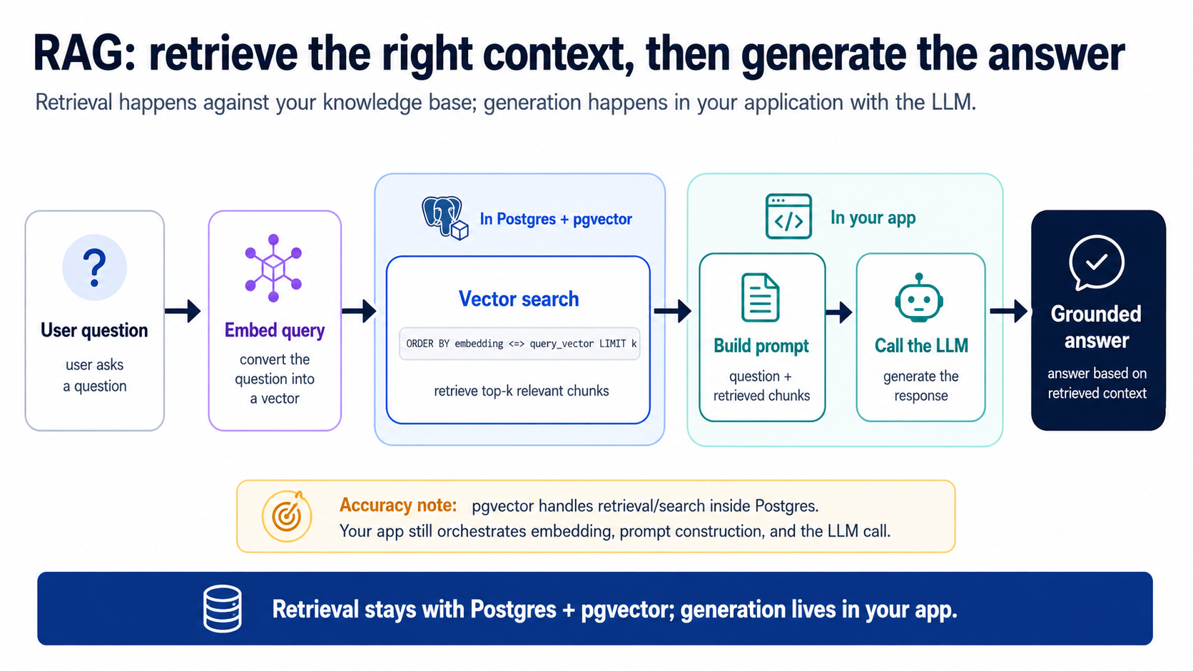
The loop has two stages, and the split is the whole point:
- Retrieve (in Postgres): run the Concept 8 query to pull the top k most relevant chunks (k is just how many you ask for; 5 is a fine start). This is the context-management step — fetch the signal, leave the million irrelevant rows out.
- Generate (in your app): build a prompt = system instructions + retrieved chunks + the user's question, send it to an LLM, return the answer. The agent writes this app-side glue for you; it's small.
Build it in two steps, so you see retrieval working on its own before generation wraps it. First, one housekeeping prompt so the code has a home — already true if you built the worker in Concept 6, in which case the agent will just confirm it:
Make sure this folder is a uv-managed Python project — set it up if it isn't — and keep every dependency and script going through uv.
Now the search half:
Build a
search_quotes(question)function in application code: embed the question, run our top-k semantic search againstquotes_embedding, and return the matching chunks with their source quotes. Then run it on "the city that never sleeps" and show me what comes back.
What comes back is stage 1 alone — the right chunks, found by meaning, before any answer is written. Now wrap stage 2 around it:
Now build
answer_question(question)on top: callsearch_quotes, format those chunks into a prompt as context, call the LLM, and return the grounded answer — retrieval stays in SQL, generation in app code. Then ask it a question and show me the retrieved chunks next to the final answer.
Notice what stage 1 is doing: handing the LLM exactly the context it needs and nothing else — context management, just as the opening diagram promised. If retrieval is sloppy — wrong chunks, too many, irrelevant ones — the LLM gives a bad answer and people blame "the AI." It's almost always the retrieval. Which is why Part 4 exists.
Then, in the next breath, they described a system that indexes documents, embeds queries, and retrieves relevant chunks before generating an answer. Respectfully: that is still RAG.
You have now built every step of it. Here is the whole machine on one card:
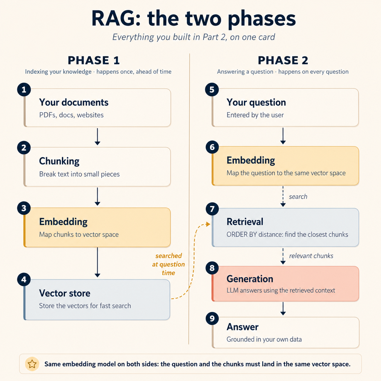
Phase 1: indexing (happens once, ahead of time):
- Your documents get broken into chunks (Concept 7)
- Each chunk gets embedded into vector space by your worker (Concept 6)
- The vectors land in Postgres, next to the data they describe (Concept 5)
Phase 2: answering (happens on every question):
- The user's question gets embedded into that same vector space
- Retrieval pulls the chunks closest to the question (Concept 8)
- Those chunks get passed to the model, which generates an answer grounded in them (this concept)
The part that trips people up on their first pipeline is hiding in one word above: same. The question and the documents have to land in the same vector space: same embedding model, same dimensions, same settings, on both sides. Embed your documents with one model and your queries with another and retrieval quietly falls apart, with no error anywhere: two models' vector spaces are simply different coordinate systems, so "closest" stops meaning "most similar." No leaderboard ranking saves you from that mismatch. (It is the model-level cousin of the expected 1536 dimensions, got 3072 error from Concept 6, except this version does not even fail loudly.)
So what actually changed since the "RAG is dead" headlines? Not the mechanism: the packaging. Agents, tool calls, and multi-step reasoning now sit on top of the same retrieve-then-generate loop. You will wrap this exact loop as an agent tool in Part 6 and hand it to an agent in Part 8: the loop does not die, it gets promoted.
answer_question() isn't only a chatbot backend — it's a tool an agent calls. In the agent chapters, retrieval becomes one of the tools a larger agent reaches for when it needs grounded facts, the same way it reaches for a calculator or a web search. RAG is the searchable context an agent draws on.
Part 3: Making search fast — indexes
Intermediate from here. Parts 3 and 4 are the tuning layer: you could ship on Parts 1–2 alone, but you won't stop there — read these for the why, then run all of them for real in Part 5, Steps 5–8. Faster (Part 3) and sharper (Part 4) are skills you'll have done, not just read.
10. Why you need a vector index (and when you don't)
Without an index, a similarity search compares the query vector to every row — an exact nearest-neighbor scan. That's perfectly accurate, and perfectly fine while you're small. As the table grows, it gets slow.
The fix is an approximate search: trade a sliver of accuracy for a large speed-up by not checking every vector. A vector index is the data structure that makes that approximation good.
The threshold that saves you from over-engineering: below roughly 100,000 vectors, exact search is often fast enough — and always correct. But the real threshold shifts with dimensions, compute size, speed target, filters, concurrency, and how often the vectors get rewritten, so have the agent benchmark before adding an index rather than reaching for one by default; add it when searches actually get slow, not before. (This mirrors the coding course's "add a rule when something goes wrong, not before.")
11. The indexes, which to use, and how to tune them
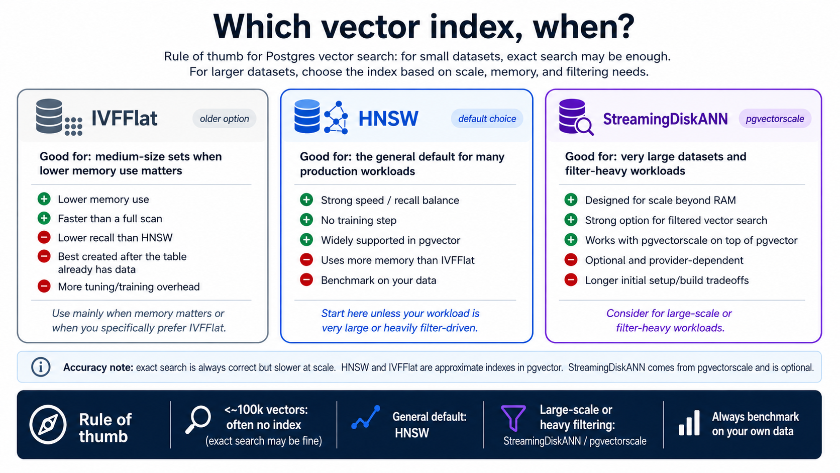
On Neon, the live choice is the middle card: HNSW is your workhorse (with IVFFlat as a legacy option). The StreamingDiskANN card is native on TigerData; from Neon, reaching it means moving to a host that ships pgvectorscale.
The agent builds the index for you — your job is to recognize what it built and confirm it fits your queries. One constraint the cards don't show: a column can hold only one vector index type, so this is a real either/or. Here's what each looks like:
-- HNSW — your default on Neon
CREATE INDEX ON quotes_embedding USING hnsw    (embedding vector_cosine_ops);

-- IVFFlat — also on Neon; legacy, needs a lists parameter; recall drifts as data grows, so periodic rebuilds
CREATE INDEX ON quotes_embedding USING ivfflat (embedding vector_cosine_ops) WITH (lists = 100);

-- StreamingDiskANN — native on TigerData; on Neon only via a pgvectorscale host
CREATE INDEX ON quotes_embedding USING diskann (embedding vector_cosine_ops);
Note vector_cosine_ops — the index must match the distance function your queries use (<=> → cosine). Mismatch this and the index silently won't help.
How to actually decide: benchmark it. HNSW has two build-time settings — m and ef_construction — that shape the graph as the index is built. They're exactly the kind of thing you never memorize: describe your real workload, and let a throwaway branch pay for the experiment. Two prompts (the row counts here are a real-scale stand-in — you'll run this exact benchmark for real in Part 5, Step 5, on a throwaway branch seeded to scale, so it lands as a skill and not a story):
We have about 2 million quote-vectors and we filter most searches by city. On a fresh Neon branch, build an HNSW index with its default settings, run ten representative searches, and report the p95 latency.
Now tune
mandef_construction: try a few settings, re-run the same ten searches on each, and recommend one — explain the tradeoff in a paragraph. Then throw the branch away.
That's the AI-engineer move: you don't memorize which settings are faster, you make the agent measure on a Neon branch and bring you a recommendation you can sanity-check against the cards above — then discard the branch at no cost. This benchmark measures speed, not recall: don't eyeball whether the results "look right" here — you judge recall the honest way, on real embeddings against your eval set (Concept 12), never by glancing at a synthetic run. (p95 latency just means the speed 95% of queries come in under — a sensible worst-case to hold the line on, but only over enough queries: think hundreds, not ten, and only after a few warm-up searches heat the branch's cache, since a fresh Neon branch serves its first reads cold from storage. Over ten cold samples, p95 is basically your single worst query.)
Row count isn't the only axis — churn is the other. How often your vectors get rewritten (re-chunking, swapping embedding models, time-decay re-indexing) is a cost of its own. HNSW takes incremental inserts and updates without a full rebuild, but heavy rewrite volume bloats the graph over time — recall drifts and you eventually need a REINDEX — and the re-embedding itself is compute you pay for. So data that's constantly rewritten can get expensive well before it's large. Tell the agent your real update pattern, not just your row count, and have it benchmark against that.
The one knob worth knowing day to day: ef_search. The build-time settings above are baked in once the index exists; the dial you'll actually touch is at query time — ef_search controls how hard a search looks: higher means better recall and slower queries, lower means faster and less accurate. The agent sets it per query; this is the line you'll see it run:
SET LOCAL hnsw.ef_search = 100; -- raise for more recall, lower for more speed
So the move is: tell the agent the recall you actually need and have it tune ef_search to hit it, not blindly max it. Then have it prove the index is doing its job: run EXPLAIN ANALYZE, check for an index scan rather than a sequential scan, and report back. Here's the difference, in the part of the output you actually read (the same 2M-vector table, with and without a usable index):
✅ GOOD — the index is doing the work
->  Index Scan using quotes_embedding_hnsw_idx on quotes_embedding
      Order By: (embedding <=> $1)
 Execution Time: 0.8 ms

❌ BAD — no index used; every row got scanned and sorted
->  Seq Scan on quotes_embedding  (rows=2000000)
      Sort Key: (embedding <=> $1)
 Execution Time: 52.4 ms
Two lines tell you which you got: the operator line (Index Scan using …hnsw… versus Seq Scan on …) and the execution time (sub-millisecond versus tens of milliseconds on the same data). Seq Scan means the index isn't being used — usually because the query's distance operator doesn't match the index, or because no index exists yet. That's the one thing to have the agent confirm before you call indexing "done."
These are the recurring ways vector search quietly breaks — and since your job is judging the agent's work, they're exactly what to watch for:
- Dimension mismatch — the column's dimensions don't match the embedding model's output.
- Vector type not registered in the client — the worker (and the search code) must register pgvector on each database connection that touches the
embeddingcolumn (register_vector), or vectors quietly round-trip as plain text: inserts and searches then misbehave with no error at all. This is the one silent-corruption mode that isn't visible in the SQL, so ask the agent to confirm it registered the type. - No index past the point where you needed one — a silent slowdown, not an error.
- Operator / index mismatch — the query uses
<->but the index is cosine, so the index is ignored. - Whole documents instead of chunks — the Concept 7 mistake; retrieval can never find anything precise.
- Skipping
EXPLAIN ANALYZE— so nobody catches any of the above until users do.
Filtering has a trap worth knowing, and it's exactly the "filter most searches by city" case in the benchmark above. An HNSW index applies your WHERE clause after it scans its fixed candidate budget (ef_search, 40 by default), so a selective filter can leave you with fewer rows than your LIMIT and quietly drop real matches — watch for under-LIMIT result counts when you validate those searches. The levers that hold recall up are query-time, not a denser graph: raise ef_search, or turn on iterative scans (SET hnsw.iterative_scan = strict_order — off by default), or build a partial HNSW index per filter value. An ordinary B-tree index on the filter column helps too, but not by pre-narrowing the HNSW scan — Postgres uses one index per scan, so the B-tree just gives the planner an exact-distance alternative it can pick when the filter is selective enough (full recall, no post-filter loss). (StreamingDiskANN — the third card above — is built for heavy filtered search at very large scale.) On Neon, these levers plus good filter indexes carry you a long way first.
Part 4: Making search good — the advanced layer
A working RAG is not a good RAG. This is where most projects stall, and where knowing the moves separates you from someone who can only produce a demo.
12. Eval-driven development
The habit that separates a shippable system from a lucky demo. Most people start by building, then eyeball whether the output "looks right." Instead, start with the questions. Before writing anything, write down a dozen questions your users will actually ask and put them in a file. That file is your evaluation set — your yardstick for whether a change made things better or worse.
Then, whenever you change the system — a new embedding model, a different chunking strategy, an added filter — you re-run the eval set and see the effect, instead of guessing. As the app grows, the set grows with it (20, 50 questions), and you catch regressions before your users do.
The second half is decompose the problem. When an answer is bad, don't conclude "the AI is dumb." Trace the stages:
- Retrieval: did semantic search even return the right chunks? (Often the real problem is an inventory gap — users ask about something you never put in the database.)
- Context: were the right chunks passed to the LLM, or too many/too few?
- Generation: given good context, did the model still answer poorly?
Nine times out of ten the failure is retrieval, not the LLM. Fix the stage that's actually broken.
Build yours now, against whatever you've loaded — the quotes from Part 2, or your own data. First the questions — the agent drafts, you curate:
Read our source table and draft 12 eval questions a user might realistically ask — some with one obvious source row, some whose answer spans several, and a couple our data can't answer at all. Note the expected answer for each (or "not answerable"), and save them to
evals/questions.mdfor me to edit.
Edit that file before you bless it — you know your users; the agent doesn't. Then wire the harness:
Build a small harness that runs each question in
evals/questions.mdthrough our retrieve-then-generate pipeline, and for each one show: the chunks retrieved, the final answer, and whether it matches what I expected. Summarize where it's failing — retrieval or generation.
From now on, every change gets measured against it:
Run the evals and save the results as today's baseline. After our next change, re-run and show me the diff — which questions got better, which got worse.
Each eval run makes one model call per question, and you'll re-run the set many times. On a free tier you'll eventually hit the provider's daily request cap and see a 429 partway through. That's the cap, not something you broke: wait and retry, have the harness back off and retry automatically, switch to a smaller free model for routine runs, or enable billing. The exact limits move, so check your provider's dashboard rather than trusting a number.
Eval-driven development is the spine of reliable agents, not just RAG. The dedicated treatment is the Eval-Driven Development Crash Course — do it after this one.
13. Filtered search: the WHERE clause is your friend
Pure semantic search returns the globally most-similar rows. Often you want the most similar rows that also satisfy some condition. Because your vectors live next to your data (Concept 5), this is just a WHERE clause on the same query — no second system, no juggling. Five patterns cover almost everything:
| Pattern | Example use case | The added clause (sketch) |
|---|---|---|
| Metadata filter | Docs search across multiple products | WHERE product = 'CRM' AND doc_type = 'api-reference' |
| Composite filter | E-commerce recommendations | WHERE category = 'electronics' AND price BETWEEN 500 AND 2000 AND in_stock |
| Time filter | News recommender — only recent articles | WHERE published_at > now() - interval '7 days' |
| Permissions filter | Internal RAG where users see only what they're cleared for | WHERE clearance_level <= $user_level |
| Geospatial filter | "Recommend things within 5 km" (add PostGIS) | WHERE ST_DWithin(location, $point, 5000) |
Each is the same shape: ORDER BY embedding <=> $1 with a WHERE in front. The permissions one is worth dwelling on — it's how you keep tenant A from ever retrieving tenant B's documents, enforced in the database rather than hoped for in application code.
Add an optional city filter to our semantic search. On a Neon branch, add a B-tree index on the
citycolumn, make sure filtered queries stay fast, and show me the before/after latency on our eval set.
14. Hybrid search: meaning and keywords
By 2026 hybrid search is the strongest candidate upgrade for serious retrieval — a candidate you confirm on your eval set, not a default you ship blind. The idea: run keyword search and vector search, then merge. Each covers the other's blind spot — vector search understands paraphrase but underweights exact rare terms (a product code, a person's name); keyword search nails the exact term but misses meaning. Postgres does both natively — keyword search via full-text search (tsvector), vectors via pgvector — so it stays one database and, often, one query.
(One note on the keyword side: this course uses Postgres's built-in keyword search (tsvector), which is already there and good enough for most data. A newer extension, pg_textsearch, does stronger BM25 ranking — the same method Elasticsearch uses — and comes pre-installed on TigerData. Switch to it only if your evals show the built-in search missing good results. The RRF step below stays exactly the same either way.)
The shape that's become standard:
- Retrieve from both, over-fetching — say the top 20 from keyword and top 20 from vector — so the merge has signal to work with.
- Fuse with Reciprocal Rank Fusion (RRF). RRF merges the two ranked lists by position, not score — which sidesteps the real headache that keyword scores and cosine distances live on completely different scales and can't be averaged sanely. It's a few lines of SQL and needs no model.
- (Optional) rerank the top candidates with a cross-encoder — a small model that scores each query–chunk pair directly. This is the precision step: RRF picks a good pool of ~100, the cross-encoder orders the final handful you hand the LLM. Add it only if your evals say the lift is worth the extra latency.
The shape the agent produces (yours to read, not type) — it will have added a ts full-text column beside the vectors first — two ranked lists fused by RRF, all in one query:
WITH kw AS (   -- keyword side: full-text search, ranked
  SELECT id, row_number() OVER (ORDER BY ts_rank_cd(ts, plainto_tsquery($1)) DESC) AS rank
  FROM quotes_embedding WHERE ts @@ plainto_tsquery($1) LIMIT 20
),
vec AS (       -- vector side: semantic search, ranked
  SELECT id, row_number() OVER (ORDER BY embedding <=> $2) AS rank
  FROM quotes_embedding ORDER BY embedding <=> $2 LIMIT 20
)
SELECT id, SUM(1.0 / (60 + rank)) AS score      -- RRF: k = 60, summed across both lists
FROM   (SELECT * FROM kw UNION ALL SELECT * FROM vec) r
GROUP  BY id ORDER BY score DESC LIMIT 10;       -- $1 = query text, $2 = query vector
Reading it: kw returns the top 20 by keyword match and vec the top 20 by meaning, each row tagged with its rank in that list (1 = best). The final query adds up 1 / (60 + rank) for every row across both lists — so a row near the top of either list scores well, and a row that lands in both wins. The 60 (the standard RRF constant) stops any single high rank from dominating, and because it works on positions, you never have to reconcile keyword scores and cosine distances on different scales.
Add full-text search over the
quotecolumn alongside our vector search, fuse the two with RRF, and run our eval set vector-only vs hybrid. Tell me which questions improved and by how much.
Hybrid search wins most on queries that mix a concept with a specific term — "what did Truman Capote say about the city" needs the name matched exactly and the meaning understood. Whether it actually helps your data, and by how much, is a question only your eval set can answer — so measure vector-only vs hybrid before taking on the extra moving parts.
15. Multi-tenancy and text-to-SQL
Two more you should recognize even if you don't build them today.
Multi-tenancy. If you're building SaaS, each customer's data must stay walled off from every other's. There's a ladder of isolation, from loosest to strictest:
| Approach | Isolation | Cost / complexity | Typical fit |
|---|---|---|---|
Shared table + tenant_id filter | Weakest | Cheapest | Internal tools, low-risk data |
| Schema per tenant | Good | Moderate | The sweet spot for most SaaS |
| Database per tenant | Strongest | Highest (backups, ops) | High-security / regulated clients |
Schema-per-tenant is the usual balance: real isolation, one database to operate. Either way, the rule from Concept 13 stands — enforce the boundary in the database, not just in your app code. The cleanest Postgres mechanism is Row-Level Security (RLS): you have the agent write a policy once (rows are visible only where, say, tenant_id = current_setting('app.tenant')) and Postgres then applies it to every query automatically — so a single forgotten WHERE clause can't leak one tenant's vectors to another. One catch worth knowing, because it bites everyone the first time: RLS is bypassed by superusers and by the table's owner, so your app must connect as an ordinary, non-owner role (the read-only role from Part 6 is exactly right) — test the policy as that role, or you'll see no isolation and wrongly conclude it doesn't work.
Text-to-SQL. Postgres holds structured data too — numbers, dates, relations. Text-to-SQL lets a user ask in plain English ("what were Q3 sales by region?") and have an agent translate it into a correct SQL query against your real tables. What makes it accurate is a well-described schema: clear table and column names, COMMENTs that explain what each one means, and a handful of example question→query pairs the agent can learn from. Give the agent that context, keep a human in the loop to review the SQL before it runs, and combine it with semantic search (for your documents) — an agent that picks the right tool per question is the foundation of a real data assistant.
Make it real on our schema in two prompts. First, have the agent prepare the ground:
Document our tables so English questions translate well: add comments to the tables and columns saying what each holds, and save a few example questions together with the SQL they should produce.
Then just ask, in plain English:
Which person has the most quotes, and how do their quotes spread across cities? Show me the SQL you'd run first — execute only after I approve.
Text-to-SQL is plan mode by another name: have the agent show the SQL first, especially anything that writes. A wrong SELECT wastes a second; a wrong UPDATE ruins your afternoon.
Part 5: A complete worked example
One task, start to finish: an empty Neon project to a working Q&A that answers from your documents. The prompts below are the whole job — type them into either tool. The method is the coding course's one move at full size: plan with a strong model, review the plan, then let a cheaper model do the routine build.
It works either way you arrive. You stay in the same postgres-ai/ folder, but the build creates a brand-new Neon project — so nothing from the quotes build is touched, whether you worked through Concepts 5–9 or jumped straight here. If the plan proposes reusing functions you already built, that's fine; judge it in review.
0. Give the build documents and a home — the base ships none, so make some (and if this folder isn't a uv project yet, this fixes that too). Paste:
Set this folder up as a uv-managed Python project if it isn't already. Then create a
docs/folder with ten short markdown files: a mini employee handbook for a fictional company — leave policy, expenses, security, onboarding, equipment.
1. Plan first — enter plan mode (Shift+Tab in Claude Code, Tab in OpenCode) with a strong model, then paste:
I have a folder
./docsof markdown files. Build a RAG system on Neon: using the Neon MCP server, create a project and adevbranch, enable pgvector, load the docs into a table, build a small embedding worker that chunks and embeds them into a companionchunkstable, and give me ananswer_question()function that retrieves and then generates. Show me the full plan and the schema before running anything.
2. Read the plan before you approve. Check: is it working on a Neon branch? Is pgvector enabled? Does the embedding worker read the API key from the environment (and is the key kept out of the repo)? Is generation in app code? If all yes, approve.
3. Execute, in three checkpoints — switch to a cheaper model (/model in either tool) for the routine build, and don't fire the whole plan blind: run it in stages, with something to look at after each. The database first:
Looks right. Proceed with the database and the worker: create the project and the
devbranch, enable pgvector, load the docs, and run the worker once. Then show me how many chunks each document produced, so I can see the documents landed.
Retrieval next — chunks before answers, same as Concept 9:
Now the search half. Build the retrieval function and run it on three questions a new employee might ask — show me only the chunks that come back, no answers yet.
If the right chunks are coming back, generation is the easy part:
Wrap
answer_question()around it. Then ask five questions a new employee would actually ask and show me the retrieved chunks next to each answer.
4. Evaluate, then iterate — some answers will be weaker than others; that's the loop starting, not a failure. Paste:
The weakest answers used irrelevant chunks. Diagnose: is it retrieval or generation? If retrieval, try a different chunking strategy on a fresh branch and re-run the same five questions.
You now have a working RAG. The next four steps are the tuning layer (Parts 3–4) — and you're going to run each one, not just read about it. Every learner does these, on the data you already have, so the depth lands as a skill. They're independent: do them in any order, skip none.
5. Make it fast, and watch the index earn its keep (Concept 11). Ten docs are too small to need an index — so you'll create the scale yourself, on a branch you throw away, and watch the search flip from slow to instant on the same data. Paste:
On a throwaway Neon branch, create a benchmark table and fill it with enough random vectors to cross the ~100k mark where an index starts to win — no embeddings or real text needed, this is purely to create scale. Make sure each row gets its own distinct random vector (a common mistake fills every row with the same vector — have the agent verify with
count(distinct embedding)). Size it to stay inside Neon's free storage; use a smaller vector dimension for this synthetic table if that helps it fit. Run a nearest-neighbour search withEXPLAIN ANALYZEand show me the plan and the time. Then build an HNSW index — raisemaintenance_work_memfor the build so it doesn't crawl — and run the identical search again. Put the two side by side: the operator line and the execution time, before and after. Then raise and loweref_searchand show me how the latency moves. Delete the branch when we're done — that reclaims the storage.
Done when: with your own eyes you've seen Seq Scan become Index Scan using …hnsw… and the execution time drop on identical data — and you've watched ef_search move the latency. That is the speed half of Concept 11, done. (Three things that look like problems but aren't: building the HNSW index over 100k+ vectors takes a few minutes, not seconds — that's expected, not a hang, and raising maintenance_work_mem for the build cuts it down sharply; using a smaller dimension for this throwaway table changes nothing about the lesson, since index-scan-vs-seq-scan and the ef_search latency dial behave the same at any dimension; and these random vectors honestly show speed, but they can't show real recall — random points have no neighbourhood structure, so a poor recall number here means nothing. Judge recall on real embeddings against your eval set, never on synthetic data. You're benchmarking the index, not your retrieval.)
6. Filter by meaning and a condition (Concept 13). Your handbook docs fall into natural categories (leave, expenses, security, onboarding, equipment) — so you can filter for real:
Tag each chunk with the category of the doc it came from. Add an optional
categoryfilter to our search. Ask "how many days of leave do I get?" twice — once across everything, once filtered to the leave category — and show me how the retrieved chunks change. Add a B-tree index oncategoryand confirm withEXPLAIN ANALYZEthat the filter uses it.
Done when: the filtered query returns tighter, on-topic chunks, and you've seen the B-tree index in the plan — the WHERE-clause-on-the-same-query payoff from Concept 5, made real.
7. Catch the exact term that meaning alone misses (Concept 14). This is where you feel why hybrid search became the default:
Put a rare exact code into one doc — say
EXP-2031in the expenses file. Ask "what is EXP-2031?" with vector-only search and show me where it ranks. Now add full-text search over the chunk text, fuse the two lists with RRF, and ask again — show me how the exact match's rank changes. Then re-run our five eval questions vector-only vs hybrid and tell me which improved.
Done when: you've compared where the code ranks vector-only vs hybrid and let your eval set show the net effect — so you decided hybrid on evidence, not because a headline told you to. (On a corpus this small, vector search may already rank a rare code near the top; the gap hybrid closes widens as the corpus grows and the rare token gets diluted among many chunks. If hybrid doesn't visibly move things here, that's the scale effect, not a failure — confirm the RRF query runs, and let the eval comparison be the verdict.)
8. Wall off one tenant from another (Concept 15). The isolation that turns this into something you could sell to two customers at once:
Tag our chunks with two pretend tenants — split the docs in half. Write a Row-Level Security policy so a session set to tenant A can only ever retrieve tenant A's chunks. Then prove it from an ordinary, non-owner database role (RLS is bypassed by superusers and the table owner, so testing as the admin role that built the table shows no isolation — use a plain read-only role instead): have the agent create that role for you (a
CREATE ROLE+GRANT SELECT, connected to withSET ROLEor a separate Neon role and connection string — not something you set up by hand), set the session to tenant A and run a search that would otherwise match a tenant-B chunk, show it never comes back, then switch to tenant B and show the mirror image.
Done when: the identical query returns different rows depending only on the tenant the session is set to, and you ran it as a non-owner role (so the wall is real). That's Concept 15's "enforce it in the database" made concrete — RLS, not a WHERE clause you could forget.
Notice the rhythm, and notice it didn't change for the hard parts: plan → review → execute → evaluate → iterate. Indexes, filters, hybrid, and tenant isolation are the same loop as the first RAG build — the only new thing each time is what you're reviewing (the schema, the worker, the index plan, the RLS policy). Master that loop and the specific SQL stops mattering, because you can always have the agent produce it and you can always tell whether it's right — at any depth, not just the easy one.
Part 6: Ship your RAG as an MCP tool
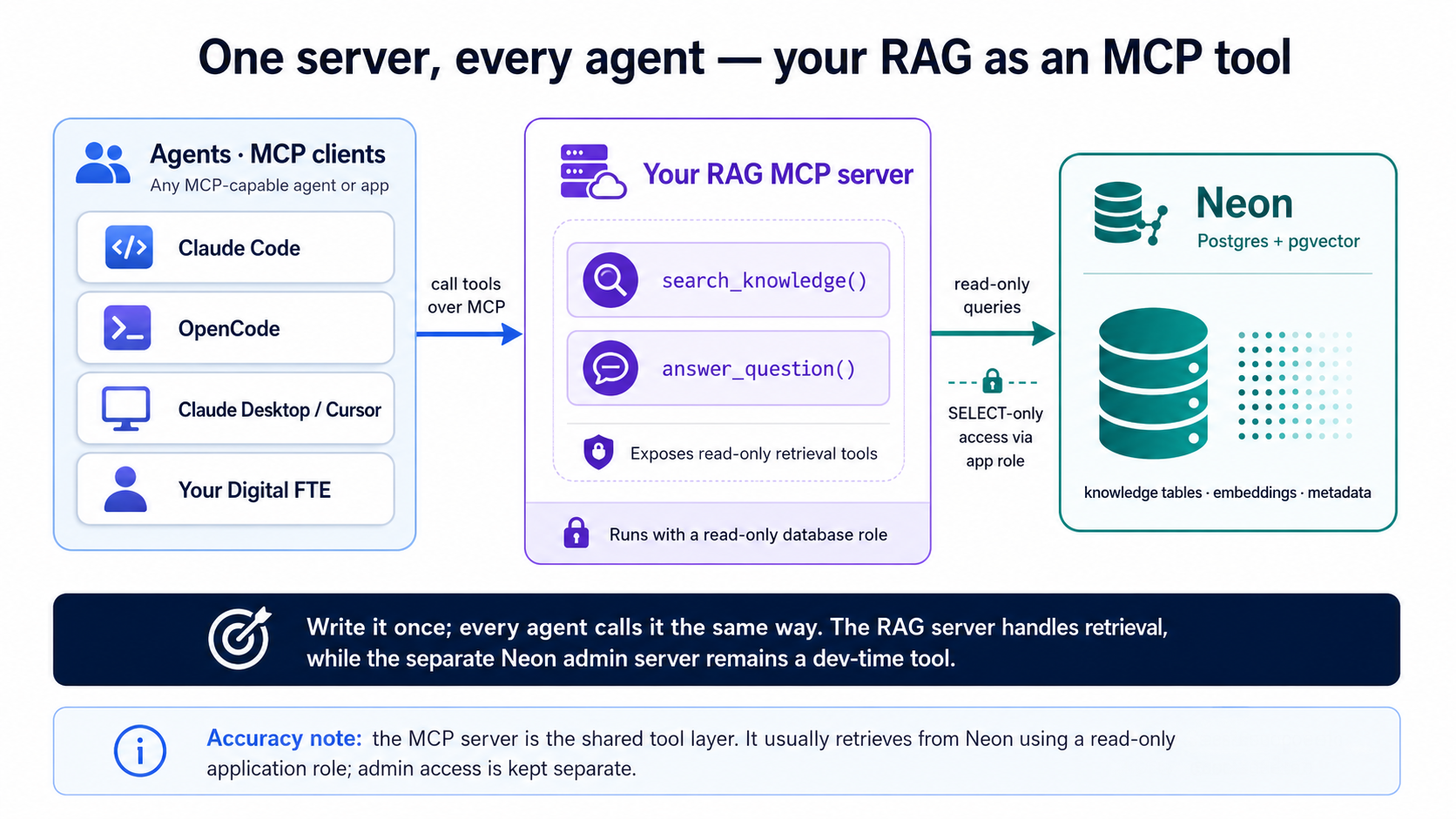
You've built search_quotes() and answer_question() (Concept 9) — and in Part 5, their document twins; this part wraps whichever you want to serve. Right now only your code can call them. Wrap them in a Model Context Protocol (MCP) server and the same retrieval becomes a tool that any agent can discover and call — Claude Code, OpenCode, Claude Desktop, Cursor, or a Digital FTE you build later. MCP is the open standard this book keeps returning to: write the capability once, and every agent speaks to it the same way.
This is the Concept 9 promise — that retrieval is the searchable context an agent draws on — made real. Your vector search stops being a feature buried in one app and becomes a reusable capability: something an agent reaches for the way it reaches for a calculator.
You've now met both, and they do opposite jobs:
- The Neon MCP server (Concept 4) is a dev-time admin tool. The client launches it locally over stdio while you build — create branches, run SQL, preview migrations. It is not for production or end users.
- The RAG MCP server (this part) is your product surface at runtime — a Streamable HTTP service you run yourself and host in the cloud, where any agent reaches it by URL. It exposes read-only retrieval — "search my knowledge," "answer from my data" — to whatever agent you point at it.
The first one builds the system. The second one is the system, offered to agents. The transport follows the role: a local dev tool the client spawns speaks stdio; a hosted product you deploy speaks HTTP. Never hand the Neon admin server to end users.
What the server looks like
An MCP server is a small program that advertises a list of tools an agent can call. With FastMCP — the standard Python library, a thin decorator layer over the official MCP SDK — each tool is just a typed function with a docstring; you don't write any of the JSON-RPC plumbing. As ever, the agent writes this — it's shown so you can judge it:
# server.py — your RAG, exposed as MCP tools (review material, not to type)
import os
from fastmcp import FastMCP
from rag import search_quotes, answer_question as rag_answer  # your Concept 9 functions —
# renamed on import so the MCP tool below can keep the public name "answer_question"

mcp = FastMCP("agent-factory-rag")

@mcp.tool()
def search_knowledge(query: str, limit: int = 5) -> list[dict]:
    """Search the knowledge base by meaning and return the closest chunks.
    Use this when you need grounded facts from the user's own data."""
    # embeds `query` in app code, runs the Concept 8 search on Neon,
    # returns [{text, source, score}, ...] — retrieval only, read-only role
    return search_quotes(query, limit)

@mcp.tool()
def answer_question(question: str) -> str:
    """Answer a question grounded in the knowledge base (retrieve, then generate)."""
    return rag_answer(question)        # the Concept 9 pipeline

if __name__ == "__main__":
    # Streamable HTTP, stateless — the production shape. The same file runs on
    # your laptop and in the cloud; stateless means no session is held between
    # requests, so it scales behind a load balancer. (host="0.0.0.0" binds all
    # interfaces so a container can route to it; locally you reach it on localhost.)
    mcp.run(transport="http", host="0.0.0.0", port=8000, stateless_http=True)
Two things matter more than the rest. The docstring is the interface — it's the text the calling agent reads to decide when to use the tool, so it must say plainly what the tool does and when to reach for it. And retrieval stays read-only: the tool runs the parameterized search from Concept 8 under a read-only database role, so a tool argument can never mutate or leak your data. The third line worth a look is the last one — mcp.run(transport="http", …, stateless_http=True) — which makes this a service you can host rather than a local subprocess; you'll run it next, then deploy the very same file.
Build it with your agent
Same discipline as everywhere else — plan, review, execute. This is also the moment the mcp-builder skill from your setup earns its keep — name it, and the agent builds the server the way the skill teaches. In plan mode:
Using the mcp-builder skill, wrap our retrieval in a FastMCP server called
agent-factory-rag. Expose two tools:search_knowledge(query, limit)returning the top matching chunks with their source and similarity score, andanswer_question(question)returning a grounded answer. Reuse our existingsearch_quotesandanswer_questionfunctions. Read the Neon pooled connection string and the model API keys from the environment, and connect with a read-only database role. Serve it over Streamable HTTP in stateless mode, so the same file runs locally now and deploys to the cloud later. Write clear, action-oriented tool docstrings — that's what the calling agent reads to decide when to use each tool. Show me the plan and the tool list before writing any code.
Read the plan, confirm the tool list and the read-only role, then approve and let it build.
Run it, then connect
Here's the shift from the Neon admin server: that one the client launches for you; this one you start, and agents connect to its URL. That's the production shape — identical whether it runs on your laptop or in the cloud. Start it:
uv run server.py
It keeps running and prints where it's serving — you'll see http://0.0.0.0:8000/mcp in the banner (0.0.0.0 just means "listening on every interface"; you connect to it as localhost). Leave it up in this terminal, open another for your agent, and register it on localhost:
claude mcp add --transport http rag http://localhost:8000/mcp
Check it with claude mcp list; reconnect mid-session with /mcp.
Add a remote block to opencode.json:
{
  "$schema": "https://opencode.ai/config.json",
  "mcp": {
    "rag": {
      "type": "remote",
      "url": "http://localhost:8000/mcp",
      "enabled": true
    }
  }
}
Then just say "use the rag tool" in a prompt — the same add → check → use flow you know from the Neon server in Concept 4, only here you point at a URL instead of a command. Try it:
Use the rag tool to answer: what did people say about New York? Show me which chunks it retrieved first.
Watch the agent call search_knowledge, get your chunks back, and ground its answer in them. That round-trip is the whole point: your data is now something any agent can reason over.
Ship it to the cloud
A local server only you can reach isn't a product yet — and an MCP tool is meant to run where any agent can call it. This is where building it stateless from the start pays off: nothing about the server changes to deploy it. You push the same server.py to any host that runs a Python service (a container on Cloud Run, Render, Railway, Fly, or your own VM), set the same environment variables there, and register the public URL instead of localhost:
claude mcp add --transport http rag https://your-host/mcp
Commit that .mcp.json and everyone who clones the repo reaches the one hosted server (Claude Code prompts them to approve it once); in OpenCode, point the same "type": "remote" block at the public URL. Add OAuth the moment more than one person connects.
Why stateless is what makes that safe: every request carries its own context, with no session held between calls — so the server shrugs off serverless cold-starts and runs as several replicas behind a load balancer without sticky sessions, and a retrieval tool, which keeps no per-user conversation, loses nothing by it. The transport you're building on — Streamable HTTP — is the stable production target; the one fast-moving detail is the exact FastMCP keyword, so let the mcp-builder skill or the live docs confirm transport="http" and stateless_http when the agent writes it. The Neon admin server stays a local dev tool either way.
A few rules to have the agent follow, and to confirm in review:
- Read-only role. The retrieval tools only ever
SELECT. Connect with a database role that can't write, so no tool argument can delete or alter data. - Parameterized queries. The query text arrives as a bound parameter, never string-concatenated into SQL — the same rule as Concept 8.
- Multi-tenancy: never trust a
tenant_idpassed as a plain tool argument. Derive it from the authenticated session and enforce it with RLS (Concept 15), so one tenant's agent can't read another's vectors. One gotcha if you ran the RLS exercise (Part 5, Step 8) on the table this server reads: the read-only role must set the tenant on every request, or RLS correctly returns zero rows — which looks like empty results with no error. Set the tenant per request, or point this server at a non-RLS table while you're still learning. - Trust the config. A local MCP server is a command another machine runs. Only register servers — and only open
.mcp.json/opencode.jsonfiles — you trust; a project config can launch a process on your machine.
And the retrieval is only ever as good as the data behind it, so your eval set still rules the day: point it at the MCP tool and you're measuring the exact thing your agents will experience.
Part 7: Where it runs
| Where | Best for | Notes |
|---|---|---|
| Neon (this course) | From first build to production | Serverless Postgres, pgvector built in, instant branching, autoscaling. You operate nothing. |
| Neon branches | Dev, preview, evals, benchmarks | Each branch is an instant clone — build on dev, preview, commit to the default branch. |
| TigerData Cloud | A full-stack alternative to Neon | "Agentic Postgres": pgvector + pgvectorscale native, Tiger MCP, instant zero-copy forks. Pick it for StreamingDiskANN scale and filtered search without ever migrating. |
You are not locked into any of these. What you learned is plain Postgres plus pgvector, with the embedding work in a worker that runs outside the database — so the skill isn't Neon-specific. The same schema, the same worker, and the same queries run on any Postgres host: Supabase, Xata (also Postgres with pgvector), Amazon RDS, Azure Database for PostgreSQL (pgvector plus a managed DiskANN vector index for scale), or your own CloudNativePG cluster on hardware you control.The same schema, the same worker, and the same queries run on any Postgres host: Supabase, Xata (also Postgres with pgvector), Amazon RDS, Azure Database for PostgreSQL (pgvector plus a managed DiskANN vector index for scale), or your own CloudNativePG cluster on hardware you control.
How to actually choose a host (once you outgrow the free tier)
Don't choose on price-per-gigabyte from a tutorial; choose on workload shape, then check the bill against your traffic.
- Bursty or idle-heavy (a side project, a low-traffic assistant, dev and eval branches): a metered serverless host that scales to zero — like Neon — only charges while you're actually running. Long idle stretches cost almost nothing.
- Always-on, steady traffic (a service that never sleeps): a flat instance price is usually simpler and cheaper than a meter that never stops ticking. Scale-to-zero stops helping the moment something keeps the database awake — including an embedding worker that polls constantly (see the worker note above).
- A fleet of databases, or data-sovereignty needs: self-hosting (CloudNativePG on your own cluster) makes the marginal cost of the next database roughly zero, at the price of running it yourself.
Two things that decide it more than the sticker rate: whether the free tier needs a credit card (it often doesn't, which matters for students), and whether the upgrade path is a smooth ramp or a cliff (a jump from a few dollars to several hundred at the next tier is a real cost, not a detail). Verify both on the provider's current pricing page — these numbers move, so this course names no figures on purpose.
A few production realities worth flagging to your agent up front:
- The embedding worker is a real process — it has to be running for embeddings to stay in sync. In production it's a service you deploy and monitor, not something you start by hand.
- Migrations: do schema and worker changes on a Neon branch, preview them, then commit to the default branch — the agent drives this through the Neon MCP's migration tools. Versioned, reviewed, reversible, and never an ad-hoc edit against production.
- Cost lives in the embedding calls and the generation calls, both of which hit external model APIs. Batch where you can, cache where you can, and use the model-matching habit — a cheap model for routine generation, a strong one where quality matters.
- Scale-to-zero vs the worker. Neon scales the database to zero when idle to save money — but an embedding worker that polls constantly keeps it awake, quietly defeating that. For low-traffic apps, have the agent set the worker to run on a schedule (or batch embeddings) rather than tight-polling, so you actually get the savings.
- Use the pooled connection string for app traffic. Neon's pooled endpoint (the
-poolerhost, PgBouncer in transaction mode) is built for the many short-lived connections serverless and high-concurrency apps open. Have the agent point your RAG-serving app at it; migrations and the worker can use the direct string. - The worker runs off Neon. You can't run sidecar processes on Neon's managed compute, so the embedding worker lives on your app host, a small VM, or a scheduled job, reaching Neon over its connection string. Tell your agent where it should run.
This is the real question behind the hype, and the honest answer is usually not. If you already run Postgres, pgvector keeps your vectors next to the data they describe — one source of truth, filters and joins in the same query, no second system to sync, secure, and pay for. HNSW comfortably covers the ~100k–10M range, and pgvectorscale's StreamingDiskANN extends past a billion vectors, so raw scale is rarely the deciding factor it once was. For most applications, Postgres is the vector database.
The big money agrees: in 2025 over a billion dollars went into Postgres companies, and both Databricks and Snowflake bought their way in — Databricks taking Neon, Snowflake taking CrunchyData. That's a good sign, but it isn't proof: the companies making this case also profit from it. The numbers they report are striking — pgvectorscale's DiskANN index is benchmarked at around 28x lower p95 latency and 75% lower cost than Pinecone at the same recall, and about 11.4x more throughput than Qdrant at 50 million vectors; pgvector with HNSW serves tens of millions of vectors at sub-100ms p99; and one team that consolidated four databases into one Postgres measured 350x faster queries. Treat these as vendor and case-study figures, not guarantees — they tell you the ceiling is high, not what your workload will do. Trust your own benchmark over anyone's headline.
A dedicated store (Pinecone, Weaviate, Qdrant, Milvus, and others) earns its place when you've measured a need it meets and Postgres can't — say, very high query throughput at billion-plus scale, a specific recall/latency target your benchmarks show pgvector missing, or a fully managed vector service you'd rather rent than operate. Those are real cases; they're just the minority. The trap is reaching for one by default because a tutorial or a headline did. Decide it the way you decide indexes (Concept 11): let your eval set and a benchmark on your real workload — including its churn — make the call, and weigh the standing cost of a second system against the gain it actually delivers.
Part 8: Hand it to an agent
You've built retrieval and wrapped it as a tool (Part 6). The natural next move is an agent that uses that tool to get real work done — which is exactly where the Build AI Agents crash course picks up. You don't rebuild any of this there; you hand the agent the tool you already have.
Here's the whole bridge in one idea. That course teaches the agent loop with the OpenAI Agents SDK: an Agent is a model equipped with instructions and tools, and a Runner drives the model → tool → model loop until the job is done. Your RAG is one of those tools. Where this course ends — a callable search_knowledge / answer_question — is where that one begins.
Two ways to connect what you built (the agents course covers the loop; you just supply the tool):
- As the MCP server from Part 6. The Agents SDK can consume MCP servers directly, so you point the agent at your
agent-factory-ragserver and its tools appear in the agent's toolbox automatically — the same server you already registered in Claude Code and OpenCode. - As a function tool. If you'd rather keep it in-process, wrap the same read-only query in the SDK's
@function_tool— that course's native tool style. Same retrieval, expressed as a Python function the agent can call.
The deeper bridge: memory vs. knowledge. The agents course frames every agent around two questions: what it can draw on (state) and what it's allowed to do (trust). One kind of state is memory — what it recalls from the running conversation, which that course handles with sessions. Your RAG provides the other kind: knowledge — durable, searchable context it can look up, across far more data than fits in any window. Sessions hold the chat; your Postgres + pgvector holds everything the agent might need to retrieve. An agent wired to both can remember what was just said and look up what it never knew — and the "fetch only the relevant chunks, leave the million irrelevant rows out" discipline from this course is exactly what keeps that retrieved context from flooding the window. Same throughline, now serving an agent instead of an app.
In the book's language, that knowledge half is the agent's system of record — the ground truth it reads from (retrieval), writes to (the worker keeps it current), and verifies against (your eval set). It is what turns a fluent guesser into an agent that executes.
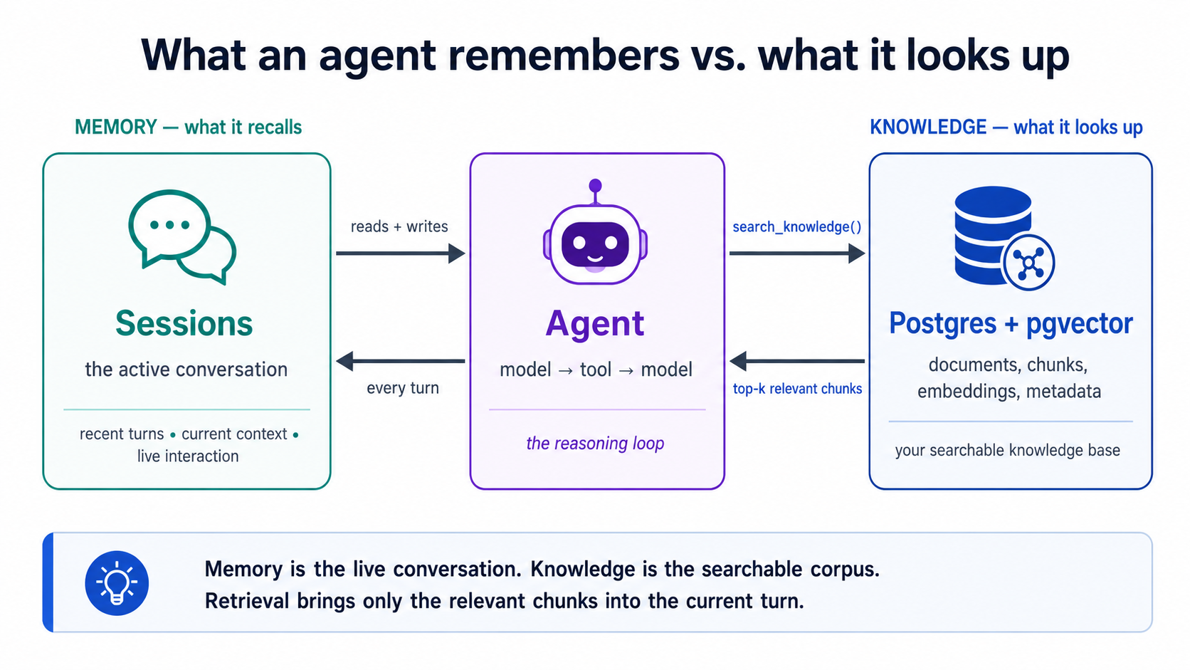
Wire it the way you built everything else — through the agent. In plan mode:
Scaffold the minimal agent from the Build AI Agents crash course (OpenAI Agents SDK — an
Agentplus aRunnerloop). Give it exactly one tool: our retrieval. Either connect it to theagent-factory-ragMCP server from Part 6 sosearch_knowledgeandanswer_questionshow up as tools, or wrap the same read-only query as a@function_tool— recommend which fits and say why. Leave the agent's own mechanics (sessions, guardrails, model routing) to that course; here, just prove the agent can call our retrieval and ground an answer in it. Show me the plan first.
Approve it, run a question that forces the tool call, and watch the agent retrieve from your Neon (or TigerData) database and answer from it. That's the handoff: Build AI Agents teaches the loop, the guardrails, the sessions, and the deployment; this course gave the agent something true to say. Your eval set crosses over intact — it still measures the retrieval the agent now depends on.
Where to go next
You now have the 80%: you can turn Neon into a vector database, build a grounded RAG system, choose an index on evidence, and improve retrieval with filters, hybrid search, and evals — all by directing an agent and judging its work.
- Make it reliable: Eval-Driven Development Crash Course
- Make it an agent: Part 8 bridges your RAG tool into an agent; the full loop, guardrails, sessions, and deployment are in Build AI Agents
- Make it a product: turn the assistant into a deployable Digital FTE
The throughline never changes: right information, right moment, irrelevant information out. You learned it for your agent. Now you can build it for everyone else's.